Abstract

This paper describes the development and application of market signals derived from the term structure of VIX futures. Current focus in financial markets is primarily on the VIX. However, this is limited to measuring the 30-day implied volatility of the S&P 500. Tracking synchronous changes in the term structure of VIX futures helps in understanding volatility beyond the 30- day window, providing a more comprehensive view. The application of this method, to follow movements of the VIX along with the term structure of VIX futures in a single frame, is demonstrated through a unique visualization tool.

Three examples of the application of this tool are presented along with sample forward 1- and 3- month returns, where applicable. The first application is in identifying suitable S&P 500 market entry points following corrections exceeding 10 percent. The second instance demonstrates the value of this tool to identify divergences in movements between VIX and the term structure during S&P 500 corrections less than 10 percent. Such divergences serve as suitable entry points in the S&P 500. Finally, the value of this tool in providing timely alerts to volatility short sellers, in advance of potential VIX spikes, is also discussed.

Introduction

The VIX® Index was developed by Robert Whaley and introduced by Cboe Global Markets Incorporated® (Cboe®) in 1993. Originally designed to “measure the market’s expectation of 30-day volatility implied by at-the-money S&P 100® Index (OEX® Index) option prices”, the Index was updated in 2003 to measure the 30-day implied volatility of the S&P 500® Index using a calculation based on near and next-term S&P 500 put and call options. The VIX has become the de facto tool for traders, financial analysts, and the investment community to gauge the market’s expectation of volatility. However, the VIX is not directly tradeable, as it is an index.

VIX futures, established by the Cboe Futures Exchange (CFE®) in March 2004, represent futures contracts of different maturities written on the VIX and are directly tradeable and optionable. Whilst the VIX and the price of VIX futures are derived separately, they share a relationship through the term structure of VIX futures. As an example, the VIX and the term structure for the first nine-month futures are shown in Figure 1.1. An upward sloping or contango structure, when the VIX futures trade at a premium to the VIX, as seen on 26th January 2018, implies lower near-term volatility and expectations of higher volatility further into the future. A downward sloping or backwardated structure, when the VIX futures trade at a discount to the VIX, as observed on 9th February 2018, implies a higher level of market fear in the near term but an expectation that this level of fear will decrease, moving forward.

Figure 1.1: VIX Futures term structure during the 2018 market correction

Although the VIX is a measure of near-term implied volatility, what constitutes “low” or “high” volatility remains subjective. As an example, consider the chart below of the S&P 500 and VIX (Figure 1.2). Following the credit crisis of 2008-09, average values of the VIX for the period 2009 to 2011 range between 24.1-31.5 and were relatively high compared to history. However, during this period, the S&P 500 rallied from a low of 677 in 2009 to a high of 1363 in 2011. In contrast to the elevated reading of the VIX, the VIX futures term structure over the same period extracted from Speth showed that the latter was predominantly upward sloping as depicted by the green shaded area in the heat map chart (Figure 1.3). Asensio made a similar observation that “the slope of the term structure was consistently positive and steep” following the credit crisis of 2008-09. Thus, market participants relying solely on the VIX reading to re-enter the market on the basis of more “normal” volatility conditions would have missed out on the rally in the S&P 500 Index from 2009 to 2012/2013, when the VIX finally returned to pre-crisis levels (Figure 1.2).

For this reason, and as noted by Fassas & Hourvouliades, we believe “that the term structure of VIX futures embeds more information regarding the equity market dynamics than spot VIX”. Given the above observation, it stands to reason that a measure based on the term structure would provide superior value. Used in conjunction with the VIX, it could provide more timely signals, with regards to the onset and recovery from market corrections, than those based on the VIX alone.

Figure 1.2: VIX and S&P 500 Index over the period January 2005 – November 2018

Figure 1.3: Term Structure of VIX futures shown as heatmap with periods of contango color-coded green, backwardation red and flat yellow.

This paper describes the development of a method based on variance from an established reference term structure of VIX futures. Used visually in conjunction with the VIX, it serves to identify various stages in market performance. The validity of this method is tested through a bull and bear market, to determine if it provides useful market entry signals during corrections exceeding 10 percent. Its value in identifying divergences between VIX spikes and movements in the term structure of VIX futures during corrections of less than 10 percent is examined as well. Finally, the application of this method for early identification of VIX spikes, which could be of value to volatility short sellers, is discussed.

Section 2 begins with a review of available literature related to VIX and VIX futures term structure. This is followed by Section 3, where the methodology used in developing the tool is described. Section 4 discusses the application of this tool to three different scenarios in a visual format and Section 5 presents the conclusions.

Literature Review

The Significance of VIX

The Cboe Market Volatility Index (VIX) is the premier benchmark for U.S. stock market volatility. It represents a “market consensus forecast of stock market volatility over the next thirty calendar days” and is often referred to as “the investor fear gauge”. Statistically, “the VIX Implied Volatility Index is an important driver of the S&P 500 future returns”.

The Applications of VIX

VIX has acquired global acceptance as the ultimate barometer of investor sentiment since its introduction. Whaley also elaborated that the level of VIX was an indication of how much market participants were willing to pay, in volatility terms, for hedging or speculation. Giot noted that VIX could also be used as a market timing indicator, with extremely high levels of VIX being concurrent with an undervalued level of S&P 500. He observed that positive returns could be achieved, for long positions initiated, when VIX reaches extremely high levels and vice versa. Fassas & Hourvaliades also noted that high levels of VIX are usually considered a capitulation signal, indicating the undervaluation of stock prices and highlighting potential buying opportunities. The same authors note that low levels of VIX imply excessive complacency and may signal a market correction. Kaufman provides examples of trading strategies based on extreme levels of VIX. Speth observed that VIX tends to spike in response to sharp downward movements in the S&P 500 and falls more slowly in rising markets. Moran estimated that the VIX had a negative correlation of -0.7 with the S&P 500 over the past 25 years.

The Limitations of VIX

Asensio noted that forecasts of changes in the level of VIX (implied volatility) tend to overshoot realized volatility consistently, and strategies designed to profit from this phenomenon have not been successful in eliminating this arbitrage opportunity. The same author argues that this could be due to significant inflows of capital from non-professional investors via ETFs. Edwards and Preston observe that VIX today, more often than not, overstates the level of actual volatility experienced in the next 30 days. Rather than state that VIX is too low or too high, they have developed a tool to calculate expected volatility based on mean reversion of realized volatility. They found that comparing actual VIX levels with their model output enabled them to identify whether VIX was high or low and to provide indications of future realized volatility.

The Increasing Importance of VIX futures

VIX futures, established by the Cboe Futures Exchange (CFE®) in March 2004, represent exchange traded contracts of different maturities written on the VIX. While VIX and VIX futures are highly correlated, Frijns, et al. note that there is “evidence of causality from VIX futures to the VIX”. As a result, VIX futures have become “increasingly more important in the pricing of volatility” and additionally are utilized as a stock market timing tool. The shape of the VIX futures term structure, in particular, “has signaling effects regarding future equity price movements”.

The VIX Futures Term Structure

Asensio notes that the existence of a term structure implies that the market assigns different prices for different time horizons. He also observed that VIX futures were consistently overpriced relative to subsequent moves in VIX, with the forecast bias increasing substantially for shorter tenors. This bias is relatively small during periods of extreme volatility. Zhang, et al. provided a comprehensive analysis of the VIX futures market between 2004-2009. During this period, research found that the average VIX futures term structure was upward sloping, and VIX futures prices were fairly well explained using a simple stochastic volatility model calibrated to actual data.

Lu and Zhu provide a good summary of different models developed to describe the VIX futures term structure. Fassas has shown that the estimated slope measure, using the least squares method, is a sufficient gauge of the VIX futures term structure. His proposed term structure was estimated as the slope of the term structure of the first six VIX futures contracts and the spot VIX. Using a study period from March 26, 2004 to July 30, 2010 the author found that the VIX futures term structure varied significantly over time. Although the term structure tended to be upward sloping, sustained periods of downward sloping term structure were also observed. The author also found that the term structure could be mainly captured by three factors: a level factor – parallel shifts of the term structure, a twist factor – shifts in the slope of the term structure and a curvature factor – changes in the steepness of the term skew.

Using VIX Futures Term Structure for Market Timing

Fassas and Hourvouliades have studied the relationship between the VIX futures term structure and future S&P 500 returns. Their findings support the hypothesis that the term structure of VIX futures can be employed as a contrarian market timing indicator for the US equity market. Using an evaluation period between 2010-2017, they fitted a linear model of daily futures prices and spot VIX as a function of maturity based on the least squares criterion. Their model found that VIX futures embed more information regarding equity market dynamics than spot VIX. Their main empirical finding is that a negative VIX futures term structure indicates oversold stock prices and could signal attractive buying opportunities.

Speth notes that mean reversion and long-term uncertainty are drivers of VIX futures term structure, and the difference between the VIX and one-year futures could be a simple way to measure term structure. Rhoads noted that in 9 out of the 10 worst trading days of the S&P 500 in 2007, the VIX first month futures contract was up by more magnitude than the S&P 500 lost. He observed that divergence was created when the VIX rose more (and the first month futures contract rose less) than what the S&P 500 lost. Rhoads identified this as a potential buying opportunity.

McMillan noted that the “short volatility” trade relies on an upward sloping term structure in VIX futures. He also stated that knowledgeable players understand that it is timely to exit such trades when the term structure flattens or begins to slope downward.

Methodology

Data Period and Sources

The data used for analysis in this study was obtained from Quandl, Cboe and the Federal Reserve Economic Data (FRED). Table 1 below lists the source of each instrument.

Table 1: List of data sources for instruments used in this study

Daily closing prices of the instruments outlined in Table 1, covering the period 19th July 2007 to 7th October 2019, were used for the analysis. The starting point of this study was primarily dictated by liquidity considerations; in essence, although futures on the VIX were introduced by Cboe in 2004, their liquidity remained relatively low until 2007. It is important to point out that while the period from 2007 to 2009 is also a period of low liquidity by comparison (Figure 3.1), it has been included to cover both a bull and bear market, given the limited available dataset.

Figure 3.1: VIX futures Average Daily Volume 2006-2019 H1

Data Preparation

To determine outliers and erroneous values, a data check was done using Refinitiv Datastream as a separate source. No major outliers were identified, and no data cleaning was required. Convergence of first month futures with the VIX near expiry was handled by implementing the following data smoothing step. Starting five days prior to expiry (t) of each front month future (VX1), its price was recalculated as follows (1):

Process Description

Core to the development of this method is the establishment of a VIX futures reference term structure based on a representative period. The rationale here is that a baseline reference could be built from data where the predominant term structure is positively sloping, indicating an uptrend. Corrections from the uptrend could then be measured as variances from the reference term structure. To select the reference period, the chosen time range for this study is split into rallies and corrections exceeding 10 percent. After identifying such rally and correction periods, a specific rally period is chosen from among all the rally periods to calculate the reference term structure. This is then applied across all other periods to measure variances from it. Each step of the process is described in more detail below.

Identifying Rally and Correction Periods

As a rule, S&P 500 declines equivalent to or larger than 10 percent were used as cutoff points to differentiate between minor and major corrections/bear markets. The correction periods identified are summarized in the daily chart of the S&P 500 shown in Figure 3.2; the start of each correction is marked using a red vertical line in the same chart.

For each such correction, the recovery and continuation of the uptrend was identified using downtrend lines drawn from the highest high marking the end of a rally through lower highs as per classical technical analysis (TA). A break above the downtrend line would then signal a resumption of the uptrend and these are shown as green vertical lines in Figure 3.2. A total of six rally and six correction periods were identified using this method. Charts 1-6 in Appendix B show in detail how the downtrend lines were applied in each instance.

Admittedly, identifying rally and correction periods by drawing trend lines introduces an element of subjectivity into the analysis. However, the primary purpose of this method is to ensure that these periods are broadly defined using conventional TA tools, to demonstrate the comparative capability of this method during these periods. The exact dates of the rally and correction periods defined in this manner are shown in Table 1.B in Appendix B.

Figure 3.2: S&P 500 showing rally and correction periods identified using trendline breaks

Developing the Reference Term Structure

Having defined the rally and correction periods, the next crucial step is to establish a reference term structure. In this study, the reference term structure is estimated by taking the difference between the first and sixth month futures analogous to the suggestion of Speth. While previous studies reported in the literature reviewed include the VIX as part of the analysis of the VIX futures term structure, the present study has separated the two components in order to capture deviations in movement between the two. Variances from the reference term structure are calculated on a daily basis and this value is reported as “VRS” (Variance from Reference Structure).

Several studies have shown the term structure to be generally upward sloping in the longer term as highlighted in the Literature Review. Thus, a negative slope, caused by a spike in values of the VIX, is not sustainable for very long periods as a result of the mean-reversion feature of the VIX. Additionally, Asensio noted that the term structure during his period of study (between Jan 2006 to Nov 2012 and included a bear market), was upward-sloping for roughly 75 percent of the time.

To establish the reference term structure, a rally period is chosen from among the six rally periods described earlier. The longer the rally period, the more reliable the reference. In this particular instance, the rally period from Jan 24, 2012 to May 25, 2015 was chosen for this calculation. It also happens to coincide with the mid-range chosen for this study.

Next, the term structure curvature is examined for the first six quoted VIX futures during this period by calculating the inter-month spreads. These spreads reflect the risk appetite between months and are the highest in the front and taper off towards outer months. The calculated inter-month spreads for the reference structure are shown in Table 1.C in Appendix C, along with key statistics such as maximum, minimum, mean, median and standard deviation. The term structure is non-linear in nature with the spread between the first and the third month accounting for close to 50 percent of the cumulative total of inter-month spreads between the first and the sixth month as illustrated in Figure 3.3.

Figure 3.3: Reference intermonth spreads

The proposed linear model serves as a good approximation to measure movements in the first month futures against the sixth month and to help understand variances from term structure through the use of the visualization tool.

Defining the thresholds for VIX and VRS

Following the calculation of VRS, its application in conjunction with the VIX is facilitated through the definition of thresholds for both VIX and VRS. Thresholds represent numerical boundaries and enable identification of changes from one regime to another. For instance, a threshold established for VIX could help identify low volatility vs high volatility periods.

Similarly, a threshold established for VRS could separate an upward sloping (contango) regime from a downward sloping (backwardation) regime. Using this principle, the threshold for VIX is calculated as the mean value over the reference term structure period, whilst the VRS threshold is defined as the boundary between upward sloping (contango) and downward sloping (backwardation) when the reference term structure moves to a flat configuration. As shown in Table 1.C in Appendix C, this threshold value was determined to be 4. The corresponding VIX threshold is 15.3.

A visual analysis tool is used to track and understand movements between the VIX and VRS. This has been achieved through a color-coded quadrant chart that defines the state of the market, based on the values of VIX and VRS at any given time. The quadrant boundaries of this chart are set using the thresholds described above. The state of the market can be segregated into one-of-four regimes using these thresholds, as shown in Figure 3.4 below. These regimes are based on whether the values of VIX and VRS are above or below their respective thresholds.

For example, when VIX and VRS are both below their thresholds (“Regime 1”), low volatility conditions prevail enabling rallies. Similarly when VIX and VRS are both above their thresholds (“Regime 3”) volatility remains high both in the present and future resulting in market corrections driven by risk aversion. “Regime 2” represents conditions where VIX is above its threshold, however, VIX futures remain upward sloping (contango) thereby establishing a divergence with the VIX. These situations could present possible market entry opportunities. “Regime 4”, representing a situation where the VIX is below its threshold and the VIX futures is downward sloping (backwardation). This is unlikely to occur in practice.

Figure 3.4: Market regimes based on VIX and VRS thresholds

Results

Having established the reference term structure and divided this study into six rally and six correction periods of S&P 500 exceeding 10 percent, we can now proceed to describe the application of this tool to three specific instances. They are:

1. Identifying suitable market entry points during the end of bear markets/corrections exceeding 10 percent.
2. Market entry opportunities created during divergences between the movement of the VIX and the term structure of VIX futures, observed during S&P 500 corrections less than 10 percent.
3. Providing early warning signals to volatility short sellers ahead of spikes in the VIX.

Each of these applications is described in detail below. Additionally, the movement of the VIX vs VRS is shown in animation form in the attached link. Instructions on how to operate it are provided in Appendix D.

Click here for online access

The password to activate this animation is CMTA.

Market Entry During Bear Markets/Corrections Exceeding 10 Percent

Applying the animation to the corrections/bear market, i.e. periods 1, 3, 5, 7, 9 and 11, deviations from the reference structure are noted for both VIX and VRS as the correction progresses with the animation showing the movement of values from the lower left quadrant (“Regime 1”) to the upper right quadrant (“Regime 3”). An example of this animation on Aug 11, 2011 is shown in Figure 4.1 below.

Figure 4.1: Snapshot of tool showing S&P 500 and VIX vs VRS plot on Aug 11, 2011

The color coding of the value enables identification of the various regimes that the data traverses. The end of a correction, or bear market, results in VIX returning close to or below threshold values and VRS returning below threshold to at or near its reference term structure. Furthermore, this tool can be used to identify suitable entry points to the long side upon VRS returning back to the reference term structure or close to it – confirming an upward sloping term structure. Examples of these instances and associated returns for one and three months forward are shown in Table 2 below for all periods examined.

Table 2: S&P 500 forward returns based on return to reference term structure

Apart from one false positive signal registered during the bear market of 2008-2009 seen in Table 2, both one- and three-month returns have been consistently positive for all other correction periods 3, 5, 7, 9 and 11. Returns are also consistently higher for a three-month holding period vs one-month. The entry dates shown in the above table represent a return to at-or-near the reference term structure. In the case of period 1, the false positive on May 21, 2008 is due to VRS returning to the reference term structure while the S&P 500 had not put in a bottom. The bottom came subsequently following which VRS returned to the reference term structure a year later, on May 20, 2009. This has also been indicated in Figure 1.2. Application of this tool to bear markets will have to await more data from similar market conditions.

It may be noted that the return of the term structure to its reference is seen to overshoot it during periods 1,3 and 5 while undershooting it during periods 7, 9 and 11. This could be explained by the changing nature of the term structure prior to and after the reference period. An examination of the difference between first- and six-month futures for the various upward sloping periods 2, 4, 6, 8, 10 and 12 was done using the date of the highest high prior to onset of the subsequent correction. The results are shown in Table 3. These dates were chosen as they serve as the best representation of an upward sloping reference term structure in each instance. The results confirm that while the sixth-month futures – representing a longer-term expectation of the level of the VIX– had declined from 24.2 to 19.4 since the bear market of 2008-09, the term structure had indeed become flatter with time during the study period; this is shown by the difference between VX1 and VX6 in the last column. An adjustment for this shift can be made to this tool by dynamically moving the reference term structure period to a more recent rally period preceding the period being analyzed. A similar principle could be applied to establish the VIX threshold due to the changing nature of the VIX average as noted in Appendix A.

Table 3: Term structure shift during study duration

Market Entry Opportunities Created by Divergences between VIX and the VIX Futures Term Structure

Rhoads identified buying opportunities during S&P 500 corrections when the percentage move in VIX was higher than the correction in S&P 500 while the corresponding move in the VIX front month futures was lower. This would imply a divergence between the moves in the VIX and the VIX first month futures for the same change in the S&P 500. Further if this were the case, such a response would carry down the futures chain to the outer months impacting the term structure. This was examined in further detail in this study as described below.

Firstly, the correlation between VIX and VRS was examined for the twelve periods chosen in this study. As shown in Figure 4.2, this correlation is shown to be very high during the correction periods 1, 3, 5, 7, 9 and 11 and lower during the primary uptrend periods of 2, 4, 6 and 8. The very low correlation exhibited during period 6 could be due to it being chosen to establish the reference term structure. At the same time, the very high correlations observed during periods 10 and 12 may be indicative of increasing recent market uncertainty.

Having identified periods of lower correlation, the next step was to confirm this during the uptrend periods of 2, 4, 6, 8, 10 and 12 using the animation tool. Results show that during these periods, VIX spikes of greater than 40 percent do not result in a change in market structure with the VRS values remaining at or below its threshold in 8 out of 12 instances. Described through the animation tool, such moves in the VIX could be observed as lateral with no significant changes to VRS values. These results are summarized in Table 4.

This could be due to market perception of the nature of certain corrections in primary uptrends. It is well known according to Dow Theory that secondary downtrends do occur during primary uptrends. While such secondary downtrends, could cause spikes in the VIX, the level of fear may not extend past a short term and hence have minimal impact on the VIX futures term structure. Under these circumstances, market perception of the extent of a correction could be indirectly observed through the number of futures months impacted.

Figure 4.2: VRS and VIX Correlation during correction / bear market periods (red) and rally/bull market periods (green)

Table 4 shows the start and end of corrections during each rally period and the corresponding percent changes in the S&P 500 and the VIX. Changes to the term structure are classified according to whether they were above, at or below the VRS threshold of 4 as shown in the table. One- and three-month returns were also calculated for market entries at the end of the correction periods, representing the maximum possible return, although entry along any point in the downtrend is possible and could lead to lower returns. These results are also shown in Table 4. Of the 12 corrections identified in the primary uptrend periods of 2, 4, 6, 8, 10 and 12, eight provided firm market entry signals at the end of their respective corrections as identified through either a flat or upward sloping term structure.

Table 4: Returns from divergences between VIX and the VIX futures term structure

While all returns are positive, the long positions established when the term structure remained upward sloping –during market corrections – consistently resulted in higher returns for 3 months over one month. The results were mixed for those instances where the market structure was flat or remained upward sloping.

Lastly, Table 4 includes results for period 6, which was earlier chosen to establish the reference term structure. To minimize the effect of autocorrelation, the term structure for the five examples shown during this period was examined from raw data for the dates shown and also shown graphically in Appendix E. These charts confirm the term structure implied by VRS.

Early Warning Signals to Volatility Short Sellers

Several authors have noted that volatility implied by VIX futures consistently overestimates actual or realized volatility of the VIX as the futures move towards expiry – particularly when the term structure is upward sloping or in contango. In physical commodities, such as oil, this difference is termed as the “cost of carry”, representing storage, transportation, financing and other charges in a period of low demand and ample supply. However, in the case of VIX futures it is attributable to volatility risk which the buyer of futures is willing to pay the seller.

As this risk diminishes in upward-sloping term structure periods (which Asensio estimates to be 75 percent of the time), the seller collects the premium, as long as the term structure is retained to front month contract expiry.

Problems do arise when the VIX spikes and the term structure moves to backwardation prior to expiry. This could result in heavy losses if the short sales are not covered in time. The most notable example, described by McMillan, resulted in the closing of XIV in early February 2018. XIV was an ETF created by investment bank Credit Suisse and constructed from short sales of near term VIX futures. The same author notes that two other ETFs of a similar nature were restructured following this event.

McMillan also noted that such losses could have been averted if long positions in such ETFs were closed out as soon as the term structure moved to flat, as astute investors reportedly did. The tool developed in this study could be applied to the monitoring of such changes to term structure as shown through the animation. Using this tool, a change in the term structure from upward sloping to flat would then be represented by the data point on the animation moving to the threshold described earlier. Such a signal could be used to liquidate a short position. However, this could lead to false positive signals from time to time as also seen in the animation.

Given the explosive nature of VIX spikes at times and the corresponding losses to any short position, it may be judicious to develop a coverage strategy, partial or total. Table 5 provides a list of dates during correction periods 1, 3, 5, 7, 9 and 11 when VRS crossed its threshold indicating a shift in term structure to flat from upward sloping or contango. Variations on this theme could apply whereby a percent-tolerance could be applied to the VRS threshold before short covering is initiated. The short position could be reestablished upon VRS returning to the reference term structure.

Table 5: Suggested dates for volatility short covering based on term structure moving to flat/upward sloping

Conclusions

The development and application of a method to derive market signals from the term structure of VIX futures is described in this paper. It uses a linear model based on the first six- month futures as an approximation to generate a reference term structure during a rally period and measures variances from it in both bull and bear markets. Used in conjunction with the VIX, in an animation format, it enables visual monitoring of shifts in term structure with changing values of the VIX.

The application of this tool to three specific cases is described along with sample calculations of 1 and 3 month returns during a bull and bear market. The first example demonstrates the value of this tool in identifying suitable entry points for S&P 500 corrections exceeding 10 percent. Positive returns are observed for all cases except the bear market of 2008-2009. While many authors have recommended buying the S&P 500 on spikes in the VIX, the present tool provides further guidance on when to “buy the fear.” In the second instance, the tool is able to identify divergences in movement between the VIX and the VIX futures term structure following corrections in S&P 500 less than 10 percent in magnitude. Suitable entry points are identified with positive one- and three-month returns. The final application described is as a risk management tool in the identification of VIX spikes that volatility short sellers would find useful. The frequency of signals in the first two applications point to its value as a long-term investment tool. Its value for short sales of S&P 500 as well as its application to other market indices was not examined. However, this work could serve as a basis for future studies.

While the application of this measure is demonstrated in conjunction with the VIX, it could also be used as a confirming tool for movements in the S&P 500 along with widely used technical analysis indicators such as MACD, RSI etc.

Acknowledgements

The author wishes to acknowledge the analytical support provided by Rashpal Sohan, Quantitative Strategist and Data Scientist.

Appendix A

Historical Annual Average Values of VIX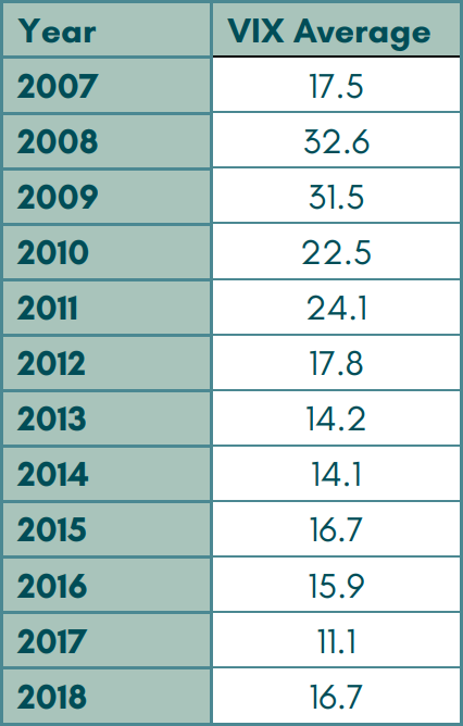

Appendix B

Identifying Rally and Correction Periods

1. Bear Market [12 October 2007 - 9 November 2009]

2. Correction [26 Apr 2010 – 9 Sep 2010]

3. Correction [2 May 2011 – 23 Jan 2012]

4. Correction [26 May 2015 – 8 Jul 2016]

5. Correction [26 Jan 2018 – 9 May 2018]

6. Correction [21 Sep 2018 – 13 Mar 2019]

Table 1.B: Correction periods with drawdowns exceeding 10 percent and associated rallies identified for study

Appendix C

VIX futures Inter-month Spread Summary Statistics and Reference Term Structure

Table 1.C: VIX Futures inter-month spreads summary statistics and reference term structure (Calculated from Period 6; See Table 1.B in Appendix B)

Appendix D

VRS vs. VIX Plot

Online Access:

Click here for online access

Instructions (Note numbers below relates to section of dashboard shown above)

1. Enter password CMTA
2. Select a period of study (rally or correction) by dragging the scrollbar. See Chapter 3 – Section 4 for additional details on what these dates relate to and how they were determined.
3. The period selected in 2 above is highlighted in the chart in the upper right-hand corner. Correction/Bear markets are highlighted in red and rallies in green.
4. Click play to animate the charts shown in 5 and 6.
5. The Chart in 5 plots VRS vs. VIX as a scatter plot for each date over the study period.
6. The chart in 6 show the corresponding move in the S&P 500 for each date over the study period.
7. Click the button in section 7 to for an analysis of the correlation between VRS and VIX for each of the relevant periods

Appendix E

VIX futures curve during Period 6 (24th Jan 2012 – 25th May 2015)

1. Rally [1 May 2012 – 1 June 2012]

2. Rally [21 May 2013 – 24 June 2013]

3. Rally [15 Jan 2014 – 3 Feb 2014]

4. Rally [16 Oct 2014 – 18 Sep 2014]

5. Rally [5 Dec 2014 – 16 Dec 2014]

---

Shared content and posted charts are intended to be used for informational and educational purposes only. The CMT Association does not offer, and this information shall not be understood or construed as, financial advice or investment recommendations. The information provided is not a substitute for advice from an investment professional. The CMT Association does not accept liability for any financial loss or damage our audience may incur.

---